| Oct 30, 2020 |
Nanomechanical indentation measurements with force spectroscopy |
| (Nanowerk Spotlight – Application Note) In the realm of nanomechanical measurements, AFM is especially suited to working with soft materials due to its piconewton force resolution and sub-nanometer vertical displacement accuracy. |
| One of the most popular AFM-based mechanical measurements is through force curves, also known as force spectroscopy. To perform these single point measurements, the cantilever approaches towards and retracts from the surface, contacting the surface up to a pre-defined force. The cantilever deflection is measured as a function of z-actuator movement. These force curves contain a wealth of information that can be modelled by various contact mechanics models to extract useful properties such as elastic modulus, stiffness, and adhesion. Force spectroscopy can be conducted in either air or liquid environments. |
| In addition to single point measurement at localized regions of interest, maps of force curves are also possible. This enables the correlation of localized mechanical property information with topographical or other information obtained by the various imaging methods. |
How does it work? |
| A sample force curves is shown in Figure 1 with cantilever deflection on the y-axis and z-actuator (piezo) movement on the x-axis. The force curve illustrates both the tip approaching the sample in black and the tip withdrawing from the sample in grey. For clarity, the grey withdrawing curve is drawn slightly below the black approach curve, thus preventing an overlap of the curves. The first observation is that the approach and withdrawal do not follow each other everywhere; they are hysteretic. |
| In other words, the motion of the tip on the way into the sample is not the same as the tip withdrawal motion, a fact that provides further information about the sample properties. The individual regions of the force curve are described below. |
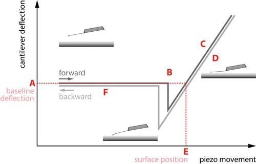 |
| Figure 1. A standard force curve. The different regions of interest are marked A through F. (Image: Nanosurf) |
| The tip approach begins with the cantilever above the surface in the region labelled A. It then snaps into contact with the surface in the region labelled B due to tip-sample interactions like capillary forces. At this point the tip is in contact with the sample and begins to push against the sample in the sloped region labelled C. The cantilever will push into the sample until a deflection or force setpoint determined by the user is reached. The tip then starts withdrawing from the sample in region D but may “stick” to the surface as it is pulled out. |
| As a result, a large adhesive dip occurs before the tip is finally able to break free from the surface and fully withdraws as shown in section F. |
| One important note about using force curves to quantify a property like elastic modulus is the requirement of careful calibration of both the tip and cantilever. One of the most important calibrations is that of the tip shape. |
| For conical or pyramidal tips this is the opening angle of the tip, for spherical tips it is the radius. For spherical tips with radii of several micrometers, optical techniques can be reliably used to measure the tip radius. |
| Available methods of tip shape calibration for small radius tips with a, pyramidal or conical tips, include direct imaging by a high-resolution technique like scanning or transmission electron microscopy or reverse imaging of the tip by imaging a surface with features that are sharper than the tip. Both are cumbersome and still imperfect since none of these methods account for changes in tip geometry over time. Hence, many users prefer to trust specifications by the manufacturer. |
| It is important to acknowledge that there can be significant uncertainty in these specifications that then leads to uncertainty in the resulting elastic modulus; it is the largest source of error in this measurement. |
| The other calibrations that are required are associated with the cantilever and detector. The cantilever spring constant is most often calibrated using a method known as the “thermal method” in which a power spectrum of a thermal cantilever tune (as opposed to a piezo actuated tune) is collected. One possibility to obtain the spring constant is to model the obtained curve with the equipartition theorem. |
| Another popular way to calibrate the spring constant from the thermal cantilever tune is known as the Sader method. This method relies on a model that is based on the influence of the hydrodynamics of the surrounding medium on the cantilever motion taking the cantilever geometry into account. |
| The final calibration step is determination of the deflection sensitivity of the optical lever. This enables the conversion of volts measured on the photodetector to nanometers of cantilever deflection. It is accomplished by conducting a force curve on an incompressible sample like glass, silicon, or sapphire: The sample has to be sufficiently hard that its compression is negligible compared to the deflection of the cantilever at the applied force. When the compression of sample is negligible, the changes in voltage from the photodetector will correspond to the deflection of the cantilever. |
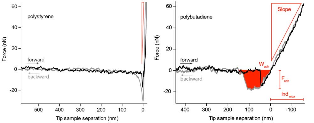 |
| Figure 2. Force curves on the harder polystyrene and the softer polybutadiene. The slope, maximum adhesion force and work needed to retract the cantilever from the sample are readily observed. (Image: Nanosurf) (click on image to enlarge) |
| As an example, individual curves collected on a blend of polystyrene (top) and polybutadiene (bottom) are shown in Figure 2. These two polymers differ greatly, both in their elastic modulus and adhesion and thus provide a great illustration of how force curves can effectively differentiate these properties on various materials. The grey curve is the motion of the tip approaching the surface while the black curve follows the tip as it retracts from the surface. |
| One main difference is the slope of the repulsive wall of the force curve (area C) where the polystyrene material clearly shows a much steeper slope than the polybutadiene, indicating that the polystyrene has a higher elastic modulus than polybutadiene. |
| Additionally, the adhesion part of the curve is also very different where the polystyrene has a larger adhesive dip (down to approx. -30 nN), indicating larger adhesion, while the area of the adhesive dip in the polybutadiene is larger, indicating a larger work of adhesion. |
| Once the force curve data has been collected, it must be modelled with a contact mechanics model to extract the elastic modulus or stiffness information. There are four main models used for AFM tip-sample interactions: Hertz, Sneddon, DMT, and JKR. The Hertz and Sneddon models do not account for any adhesion between the tip and sample, making them appropriate for samples that are not “sticky” with respect to the tip. While the Hertz model assumes a spherical tip shape and indentation smaller than the tip radius, the Sneddon model is a more general approach, including a wider variety of tip shapes such as conical and pyramidal, which are often more appropriate to describe the tip of a standard AFM cantilever. |
| Most samples do exhibit some form of adhesion on the nanoscale and thus a model that takes this into account is usually required, although the approach curves can generally still be described by the Hertz and Sneddon models. |
| The DMT model adds long range attractive forces to the Hertz area to account for adhesion outside the contact area. In the DMT model, the slope of the repulsive wall (region D) is fit to extract the elastic modulus. The JKR model accounts for stronger adhesion that occurs within the contact area; this model also accounts for the hysteresis in tip approach and withdrawal from the sample. A modified version of the JKR model called the 2-point JKR model is often used to extract the elastic modulus and it models the adhesive portion of the curve (region E). |
Applications |
| Individual force curves can be collected in an array on the sample creating a “force map” where a force curve is collected at each pixel and mechanical properties can then be extracted from each force curve to create corresponding maps of properties such as adhesion or elastic modulus. A force map was collected on epithelial cells. From individual force curves the maximum adhesion force was extracted and curves were fitted for the elastic modulus data. |
| The adhesion map is shown in Figure 3, where the adhesion was “painted” onto the 3-D topography to optimize visualization of this sample. The sample height was calculated from the fitted contact point of each force curve to get a so called zero-force sample topography. A fairly homogenous value of adhesion is found across the cell surface. The adhesion is further quantified through the histogram which shows that most occurring adhesion has a force of approximately 0.15-0.20 nN. |
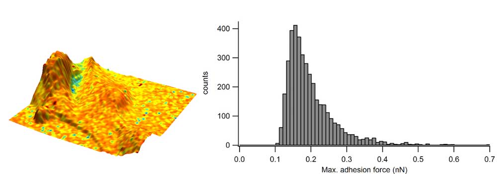 |
| Figure 3. Adhesion overlaid in colour on the 3D representation of the sample height and corresponding adhesion distribution as a histogram. (Image: Nanosurf) (click on image to enlarge) |
| A map of the elastic modulus is shown in Figure 4, where this time the elastic modulus has been “painted onto” the 3-D topography and shows a heterogeneous elastic modulus over the cell surface. The red areas show low elastic modulus values and bright purple illustrates high elastic modulus values. The histogram further quantifies these values and reveals that the taller areas of the cells have an elastic modulus below 5 kPa surrounded by a surface with an elastic modulus peaking between 10-15 kPa. |
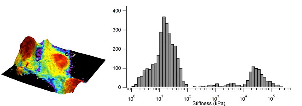 |
| Figure 4. Elastic modulus overlaid in colour on the 3D representation of the sample height and corresponding elastic modulus distribution as a histogram. (Image: Nanosurf) (click on image to enlarge) |
| Another example of force spectroscopy is to measure the properties of hydrogels, an important class of materials with applications in the medical and consumable industry. Hydrogels are comprised of a network of polymer chains with high water content and have a range of uses. Because these materials are so soft – on the order of few kPa – and must be hydrated, they are challenging to measure with any method besides AFM. |
 |
| Figure 5. Elastic modulus distribution of four hydrogels with different concentrations of gelatine. (Image: Nanosurf) (click on image to enlarge) |
| The data from four different hydrogel materials with varying gelatin concentrations that have been measured with force curves in situ under an aqueous solution is shown in Figure 5. Histograms of the moduli are shown where the colored histograms represent different 30 µm x 30 µm areas on the sample, and the grey bins represented an aggregated histogram of all the individual regions, which has been fitted to a single or double Gaussian distribution in the black line. |
| The first trend observed is that materials with the larger hydrogel component are stiffer, ranging from a material that was 0.8% gel with an elastic modulus of 24 kPa to a material that was 0.2% gel and had an elastic modulus of approximately 1 kPa. Secondly, the materials show a wider variation in elastic modulus from different probed areas, reflecting a spatial heterogeneity in gel composition in the sample, underscoring the need to repeat these measurements on large spatial scale. |
Summary |
| Taking advantage of its piconewton force and sub-nanometer displacement resolution, AFM is uniquely suited to measure nanoscale mechanical properties, especially when it comes to soft materials. Force spectroscopy is a useful nanomechanical technique to obtain both single point measurements and maps of important mechanical properties such as stiffness (elastic modulus) and adhesion. |
| Cantilever and tip calibrations coupled with contact mechanics models enable the full analysis and interpretation of individual force curves. The application of force curves to a wide variety of materials is demonstrated here including measurements of polymers, cells, and hydrogels. |
| Provided by Nanosurf AG |

Become a Spotlight guest author! Join our large and growing group of guest contributors. Have you just published a scientific paper or have other exciting developments to share with the nanotechnology community? Here is how to publish on nanowerk.com. |
